Density and Sparsity: A View of Warsaw

Maps Then, Maps Now

Keys, license, Google Maps. It is increasingly rare for drivers to shift out of park before typing in an address in a web mapping app. We turn on our phones, the nearest satellite pinpoints our position and beams us our geolocation. Frequent app updates ensure we know exactly our whereabouts.

There is a brief moment that occurs after we open our Google Maps app. In the millisecond before an above satellite triangulates our position and the map zooms in on our location, we see a wider view of our surroundings complete with roads, rivers and bridges. It’s in this brief moment that we remember how aesthetic our surroundings look when mapped from above.

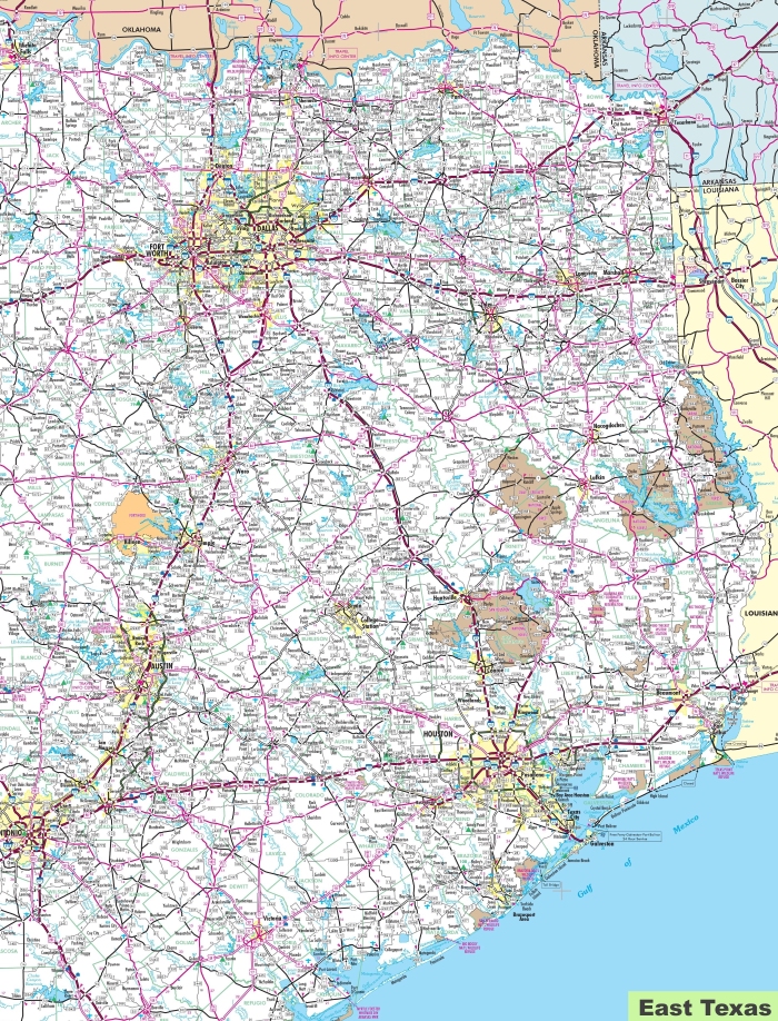
Physical maps have become a novelty. It’s hard not to admire the artistic quality of a map such as this one of Eastern Europe or this Soviet map of Manchester England. We may smirk at their uselessness now, but there is something pleasing about opening an old atlas roadmap and gawking at the byzantine tangle of lines that crisscross and intertwine.

One can’t help but think that we are missing something in the hyper-local focus of the satellite imagery which holds our hand and guides us to our location.

In the digital age, however, one can still behold the everyday elegance of a map. Who hasn’t pinned their location, zoomed out as far as they can on Google Maps until the entire round Earth is visible, and then zoomed in little by little as the continents, surrounding mountains, bridges and roads and finally your house come into view?

Warsaw to Behold

I am reminded of this magic when creating maps using software. I made a map of Warsaw recently as a gift. I planned to plot some of the highways in one color, and then use different colors for the main geographical features of the city (blue for the Wisła river that runs through the city, green for Powązki cemetery and Ujazdowski park).

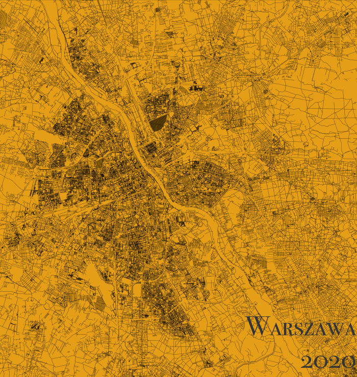
In the process, I reminded myself just how little is needed to create a map that captures the essence of the city. I created the following map of Warsaw using only highways, residential streets, pedestrian paths and bike lanes:

Without defining the natural landmarks in any way, the roads and lanes are able to capture the main characteristics of the city — the bends of the river, the dense network of pedestrian paths in the lush parks of the northwest Wola district, the large square of Brodnowski cemetery in the northeast district of Targówek.

It illustrates a simple but elegant principal in creating maps: the more dense the urban landscape, the more sparse your maps can be. You don’t need to plot much detail before it becomes obvious how the city conforms to the shape of the land.

The opposite is also true. When looking at the open fields south of Warsaw, it becomes apparent that in rural settings more natural detail is needed to give contour to the map. In the less populous city outskirts, the orange backdrop engulfs the streets and the towns. More detail is needed to capture the land and the surroundings.

While the handcrafted nature of maps may now be a lost art, digital maps can be just as inventive as the framed antiques that adorn your living room. They can also be just as laborious to make — this minimalist map was the result of endless tweaks and revisions to the R code below:

library("osmdata")
library("ggplot2")
require("sf")

export_path = "~/"
file_name = "warsaw_map.png"

###Get Base Warsaw Map

waw = getbb("Warsaw, PL")


###Get Streets

highways = waw %>%
  opq()%>%
  add_osm_feature(key = "highway", 
                  value=c("motorway", "trunk",
                          "primary","secondary", 
                          "tertiary","motorway_link",
                          "trunk_link","primary_link",
                          "secondary_link",
                          "tertiary_link")) %>%
  osmdata_sf()



ggplot() +
  geom_sf(data = highways$osm_lines,
          aes(color=highway),
          size = .4,
          alpha = .65)+
  theme_void()



streets = waw %>%
  opq()%>%
  add_osm_feature(key = "highway", 
                  value = c("residential", "living_street",
                            "service","unclassified",
                            "pedestrian", "footway",
                            "track","path")) %>%
  osmdata_sf()


ggplot() +
  geom_sf(data = streets$osm_lines,
          aes(color=highway),
          size = .4,
          alpha = .65)+
  theme_void()


color_roads = rgb(0.42,0.449,0.488)
ggplot() +
  geom_sf(data = streets$osm_lines,
          col = color_roads,
          size = .4,
          alpha = .65) +
  geom_sf(data = highways$osm_lines,
          col = color_roads,
          size = .6,
          alpha = .8)+
  theme(legend.position = F) + theme_void()


###Final Map (with cool coloring)

color_roads = rgb(0.92,0.679,0.105) 
color_roads

color_background = "#000000"
color_background

final_map = ggplot() + 
  geom_sf(data = streets$osm_lines,
          inherit.aes = FALSE,
          color=color_background,
          size = .4,
          alpha = .65) +
  geom_sf(data = highways$osm_lines,
          inherit.aes = FALSE,
          color=color_roads,
          size = .6,
          alpha = .65) +
  coord_sf(xlim = c(min(waw[1,]), max(waw[1,])), 
           ylim = c(min(waw[2,]), max(waw[2,])),
           expand = FALSE) +
  theme(legend.position = F) + theme_void()+
  theme(panel.background = element_rect(fill = color_roads))

final_map

gc()
ggsave(final_map, 
       filename = paste(export_path, file_name, sep = ""),
       scale = 1, 
       width = 18.5, 
       height = 24.5, 
       units = "in",
       dpi = 500)